Comparison with RadVel#
simppler is very much inspired from the RadVel package.
The goal when writing simppler was actually to test the underlying simpple package on a real use-case, and RadVel seemed like a good comparison (in part because I am familiar with its codebase).
This notebook compares simppler and radvel, on the one hand to make migration between the two easier, and on the other hand to make sure there is no major performance difference between the two.
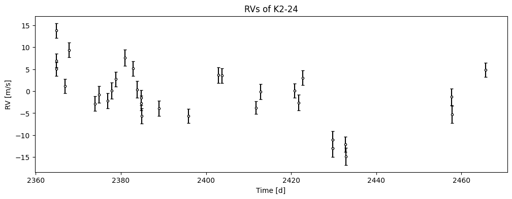
Data#
We will use the same model and data as in the K2-24 tutorial, as this example was taken from RadVel tutorial.
from pandas import read_csv
import matplotlib.pyplot as plt

url = "https://raw.githubusercontent.com/California-Planet-Search/radvel/refs/heads/master/example_data/epic203771098.csv"
df = read_csv(url, index_col=0)


t = df.t.values
vel = df.vel.values
errvel = df.errvel.values

def plot_data():
    plt.figure(figsize=(12, 4))
    plt.errorbar(t, vel, yerr=errvel, fmt="k.", capsize=2, mfc="w", label="Data")
    plt.xlabel("Time [d]")
    plt.ylabel("RV [m/s]")
plot_data()
plt.title("RVs of K2-24")
plt.show()
simppler model#
First, we build the simppler, re-using our builder function from the K2-24 tutorial.
import numpy as np
import simppler.model as smod
from simpple import distributions as sdist
periods = [20.8851, 42.3633]
period_errs = [0.0003, 0.0006]
t0s = [2072.7948, 2082.6251]
t0_errs = [0.0007, 0.0004]
def build_model(vary):
    if vary == "all":
        parameters = {
            "per1": sdist.Normal(periods[0], period_errs[0]),
            "tc1": sdist.Normal(t0s[0], t0_errs[0]),
            "secosw1": sdist.Uniform(-1, 1),
            "sesinw1": sdist.Uniform(-1, 1),
            "logk1": sdist.Normal(np.log(5), 10),
            "per2": sdist.Normal(periods[1], period_errs[1]),
            "tc2": sdist.Normal(t0s[1], t0_errs[1]),
            "secosw2": sdist.Uniform(-1, 1),
            "sesinw2": sdist.Uniform(-1, 1),
            "logk2": sdist.Normal(np.log(5), 10),
            "dvdt": sdist.Normal(0, 1.0),
            "curv": sdist.Normal(0, 1e-1),
            "gamma": sdist.Normal(0, 10.0),
            "jit": sdist.Normal(np.log(3), 0.5),
        }
    elif vary == "ecc":
        parameters = {
            "per1": sdist.Fixed(periods[0]),
            "tc1": sdist.Fixed(t0s[0]),
            "secosw1": sdist.Uniform(-1, 1),
            "sesinw1": sdist.Uniform(-1, 1),
            "logk1": sdist.Normal(np.log(5), 10),
            "per2": sdist.Fixed(periods[1]),
            "tc2": sdist.Fixed(t0s[1]),
            "secosw2": sdist.Uniform(-1, 1),
            "sesinw2": sdist.Uniform(-1, 1),
            "logk2": sdist.Normal(np.log(5), 10),
            "dvdt": sdist.Normal(0, 1.0),
            "curv": sdist.Normal(0, 1e-1),
            "gamma": sdist.Normal(0, 10.0),
            "jit": sdist.Normal(np.log(3), 0.5),
        }
    else:
        parameters = {
            "per1": sdist.Fixed(periods[0]),
            "tc1": sdist.Fixed(t0s[0]),
            "secosw1": sdist.Fixed(0.01),
            "sesinw1": sdist.Fixed(0.01),
            "logk1": sdist.Normal(np.log(5), 10),
            "per2": sdist.Fixed(periods[1]),
            "tc2": sdist.Fixed(t0s[1]),
            "secosw2": sdist.Fixed(0.01),
            "sesinw2": sdist.Fixed(0.01),
            "logk2": sdist.Normal(np.log(5), 10),
            "dvdt": sdist.Normal(0, 1.0),
            "curv": sdist.Normal(0, 1e-1),
            "gamma": sdist.Normal(0, 10.0),
            "jit": sdist.Normal(np.log(3), 0.5),
        }
    tmod = np.linspace(t.min() - 5, t.max() + 5, num=1000)
    time_base = 2420
    return smod.RVModel(parameters, 2, t, vel, errvel, basis="per tc secosw sesinw logk", tmod=tmod, time_base=time_base)

simpple_model = build_model("circular")
We will also optimize the model to ensure that we have an easy starting point for the MCMC, as our goal here is not to test sampling efficiency.
test_p = {"per1": periods[0], "tc1": t0s[0], "secosw1": 0.01, "sesinw1": 0.01, "logk1": 1.1}
test_p |= {"per2": periods[1], "tc2": t0s[1], "secosw2": 0.01, "sesinw2": 0.01, "logk2": 1.1}
test_p |= {"gamma": -10, "dvdt": -0.02, "curv": 0.01, "jit": 1.0}


from scipy.optimize import minimize

vary_p = {p: v for p, v in test_p.items() if p in simpple_model.vary_p}
res = minimize(lambda p: - simpple_model.log_prob(p), np.array(list(vary_p.values())), method="Nelder-Mead")
opt_p = dict(zip(simpple_model.keys(), res.x))
Converting from simppler to RadVel#
simppler models have a method allowing us to convert the model directly to a radvel.Posterior object.
radvel_post = simpple_model.to_radvel()
vary_p_arr = [test_p[k] for k in simpple_model.keys()]
radvel_post.set_vary_params(vary_p_arr)
print(radvel_post)
parameter                     value      vary
per1                        20.8851      False
tc1                         2072.79      False
secosw1                        0.01      False
sesinw1                        0.01      False
logk1                           1.1       True
per2                        42.3633      False
tc2                         2082.63      False
secosw2                        0.01      False
sesinw2                        0.01      False
logk2                           1.1       True
dvdt                          -0.02       True
curv                           0.01       True
gamma                           -10       True
jit                               1       True
tp1                         2070.19
e1                           0.0002
w1                         0.785398
k1                          3.00417
tp2                         2077.33
e2                           0.0002
w2                         0.785398
k2                          3.00417

Priors
------
Gaussian prior on logk1, mu=1.6094379124341003, sigma=10
Gaussian prior on logk2, mu=1.6094379124341003, sigma=10
Gaussian prior on dvdt, mu=0, sigma=1.0
Gaussian prior on curv, mu=0, sigma=0.1
Gaussian prior on gamma, mu=0, sigma=10.0
Gaussian prior on jit, mu=1.0986122886681098, sigma=0.5
Let us compare the output from the two models
plot_data()
plt.plot(simpple_model.tmod, simpple_model.forward(test_p, simpple_model.tmod), label="simppler model")
plt.plot(
  simpple_model.tmod, radvel_post.model(simpple_model.tmod) + radvel_post.params["gamma"].value, "--", label="RadVel model"
)
plt.legend()
plt.show()
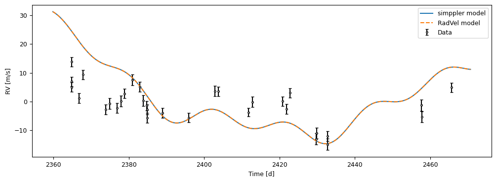
That looks good! We can now compare the execution speed of the two models.
Speed comparison#
We do not expect a big performance difference between simppler and radvel: as of writing this, the former uses the keplerian solver from the latter.
However, some performance cost may be associated with the parameter handling or how the distributions are written (this is how I realized that Scipy distributions were quite slow, and switched to custom implementations in simpple).
from timeit import timeit

timeit("radvel_post.logprob_array(vary_p_arr)", globals=globals())
89.83651479500259
For simppler, we will test with dict and array inputs to see if there is a difference.
timeit("simpple_model.log_prob(test_p)", globals=globals())
69.65383110200492
timeit("simpple_model.log_prob(vary_p_arr)", globals=globals())
75.79917559599562
As expected, everything here is fairly similar.
Sampling comparison#
We can also compare the sampling results from the two packages to ensure that they are consistent.
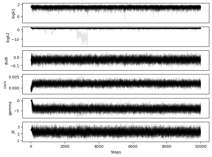
simppler sampling#
import emcee

nwalkers = 50
nsteps = 10_000
ndim = simpple_model.ndim
sampler = emcee.EnsembleSampler(nwalkers, ndim, simpple_model.log_prob)
rng = np.random.default_rng()
p0 = res.x + 1e-4 * rng.normal(size=(nwalkers, ndim))
_ = sampler.run_mcmc(p0, nsteps, progress=True)
from simpple.plot import chainplot
chainplot(sampler.get_chain(), labels=simpple_model.keys())
plt.show()
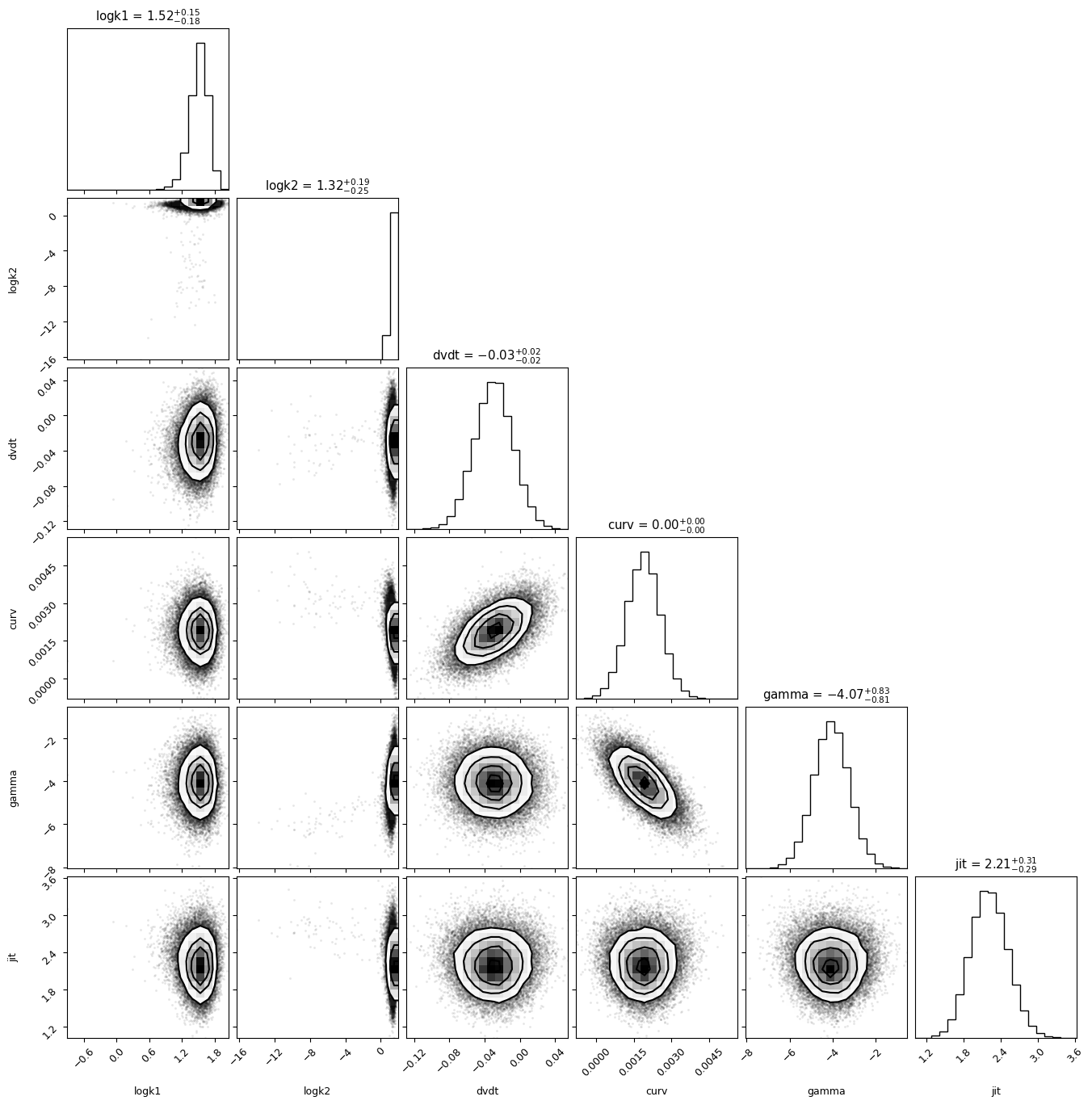
import corner
simppler_chains = sampler.get_chain(discard=2000, flat=True, thin=10)
corner.corner(simppler_chains, labels=simpple_model.keys(), show_titles=True)
plt.show()
WARNING:root:Too few points to create valid contours
radvel sampling#
import emcee

sampler = emcee.EnsembleSampler(nwalkers, ndim, radvel_post.logprob_array)
_ = sampler.run_mcmc(p0, nsteps, progress=True)
from simpple.plot import chainplot
chainplot(sampler.get_chain(), labels=radvel_post.name_vary_params())
plt.show()
import corner
radvel_chains = sampler.get_chain(discard=2000, flat=True, thin=10)
corner.corner(radvel_chains, labels=radvel_post.name_vary_params(), show_titles=True)
plt.show()
WARNING:root:Too few points to create valid contours
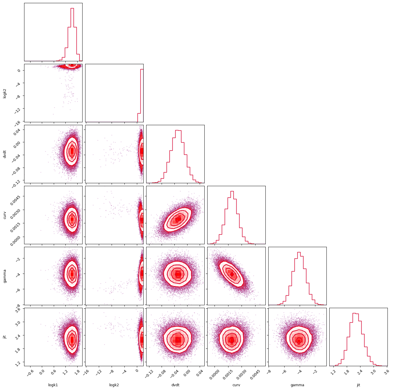
Combined corner plot#
import corner
fig = corner.corner(radvel_chains, labels=radvel_post.name_vary_params(), color="b")
corner.corner(simppler_chains, color="r", fig=fig)
plt.show()
WARNING:root:Too few points to create valid contours
WARNING:root:Too few points to create valid contours