Multi-instrument model with `simppler`#

In this tutorial, we will explore an example where we have datasets from various instruments that we want to analyze jointly in simppler.

We will replicate the “Fitting radial-velocities” tutorial from the juliet package, analyzing the TOI-141 observations presented in Espinoza et al. (2019).

import os
import radvel
import numpy as np
from pandas import read_csv
import matplotlib.pyplot as plt

plt.style.use("tableau-colorblind10")

data_df = read_csv(os.path.join(radvel.DATADIR, "rvs_toi141.dat"), sep=" ", names=["t", "rv", "erv", "inst"])
t, rv, erv, inst = data_df.t.values, data_df.rv.values, data_df.erv.values, data_df.inst.values
sort_inds = np.argsort(t)
t = t[sort_inds]
rv = rv[sort_inds]
erv = erv[sort_inds]
inst = inst[sort_inds]
tmod = np.linspace(t.min(), t.max(), num=1000)
print("Instruments:", ", ".join(np.unique(inst)))

Instruments: CORALIE07, CORALIE14, FEROS, HARPS

The observations come from four different instruments listed above. Each instrument can have its own systematic parameters: jit_{inst}, gamma_{inst}, dvdt_{inst} and curv_{inst}. Orbital parameters are shared between instruments so they do not have a suffix.

Building the model#

Let us start by building a model with all required parameters for a single-planet fit to the four instruments.

import simpple.distributions as sdist
import simppler.model as smod

P = 1.007917
P_err = 0.000073
t0 = 2458325.5386
t0_err = 0.0011

parameters = {
    "per1": sdist.Normal(P, P_err),
    "tc1": sdist.Normal(t0, t0_err),
    "e1": sdist.Fixed(0.0),
    "w1": sdist.Fixed(90.0 * np.pi / 180.0),
    "k1": sdist.Uniform(0.0, 100.0),
    "gamma_CORALIE14": sdist.Uniform(-100.0, 100.0),
    "gamma_CORALIE07": sdist.Uniform(-100.0, 100.0),
    "gamma_HARPS": sdist.Uniform(-100.0, 100.0),
    "gamma_FEROS": sdist.Uniform(-100.0, 100.0),
    "jit_CORALIE14": sdist.LogUniform(1e-3, 100.0),
    "jit_CORALIE07": sdist.LogUniform(1e-3, 100.0),
    "jit_HARPS": sdist.LogUniform(1e-3, 100.0),
    "jit_FEROS": sdist.LogUniform(1e-3, 100.0),
}
model = smod.RVModel(parameters, 1, t, rv, erv, inst=inst, basis="per tc e w k", tmod=tmod)

import simppler.plot as sp
fig, axs = sp.plot_rv(model)
plt.show()

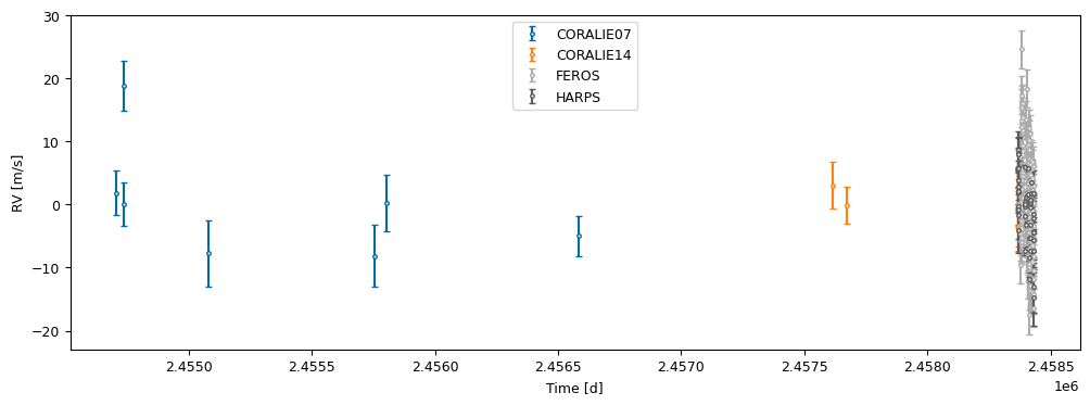
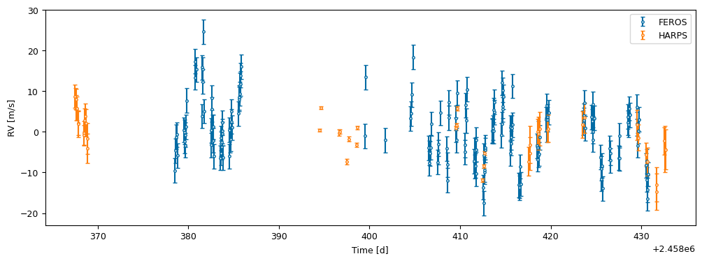
../_images/ae18f6e83d9f094d48b60b7333c3142607cad777e426846c6660edd45e9c4e1d.png

The CORALIE data is spread over a long time and very sparse. We can exclude it from the plots by specifying which instruments we want to see.

fig, axs = sp.plot_rv(model, inst=["FEROS", "HARPS"])
plt.show()

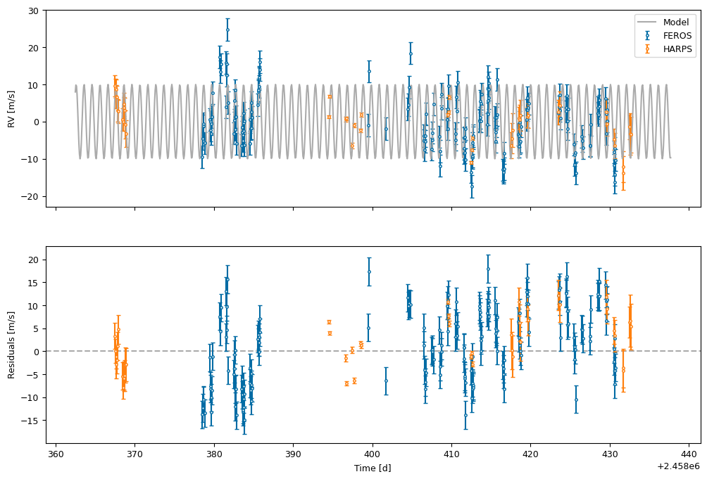
../_images/53bdf3973322a11df2cb8492cdfdff86260ae485d77a5cc362a2e5d4e04fca38.png

We can display a test model by passing the parameters argument to the plotting function.

test_p = {"per1": P, "tc1": t0, "k1": 10.0}
for inst_name in model.inst_unique:
    inst_mask = model.inst == inst_name
    test_p[f"gamma_{inst_name}"] = np.mean(model.rv[inst_mask])
    test_p[f"jit_{inst_name}"] = np.mean(model.erv[inst_mask])
fig, axs = sp.plot_rv(model, parameters=test_p, inst=["FEROS", "HARPS"])
plt.show()

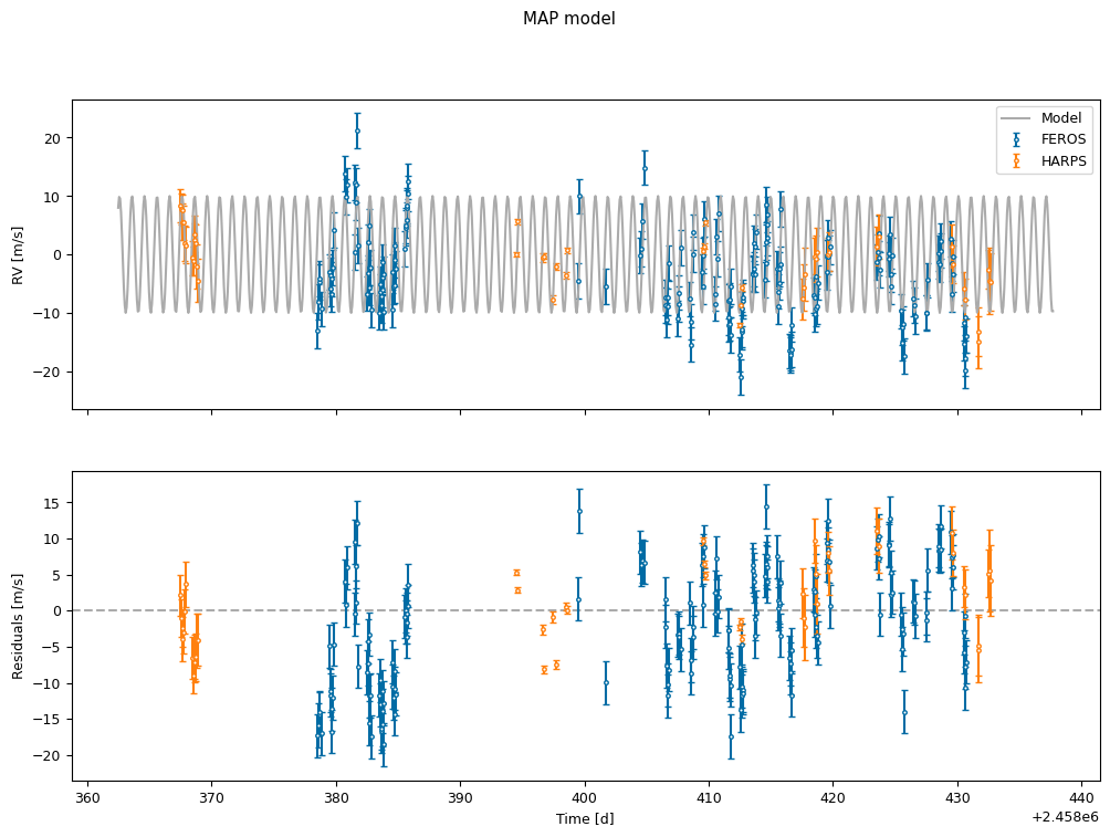
../_images/46b53bc5b5c850aa8bb88bf4d9c3f226f2745044238061fd8166e4fb23ebf279.png

MAP Optimization#

Let us now optimize our model.

from scipy.optimize import minimize
res = minimize(
    lambda p: model.log_prob(p), list(test_p.values()), method='Nelder-Mead',
    options=dict(maxiter=200, maxfev=100000, xatol=1e-8)
)

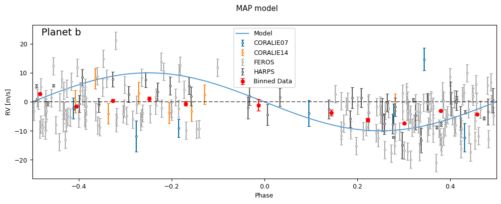
fig, axs = sp.plot_rv(model, parameters=res.x, inst=["FEROS", "HARPS"])
fig.suptitle("MAP model")
plt.show()

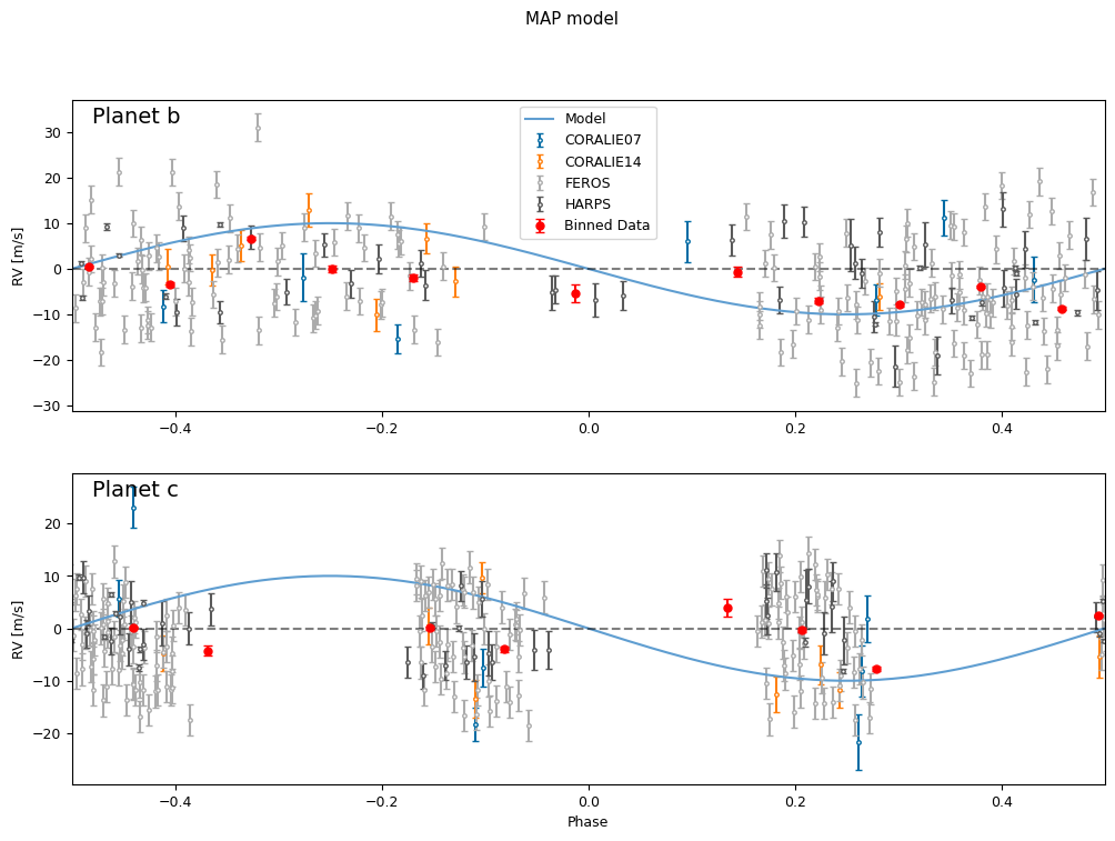
../_images/092436bf8c4a0296794624c12543a069eca0ff230d8ceb37f4bf6c2a43ec3f67.png

We can also look at the phase-folded results.

fig, axs = sp.plot_phase(model, parameters=res.x)
fig.suptitle("MAP model")
plt.show()

../_images/af13af773b8086c48232af46f9d90fc9933659f60342d5ed3d49d3031d97126e.png

Nested Sampling for a Single Planet#

To properly explore the posterior, and to derive Bayes factors for model comparison, we can use Nested Sampling with the ultranest package.

Prior Samples#

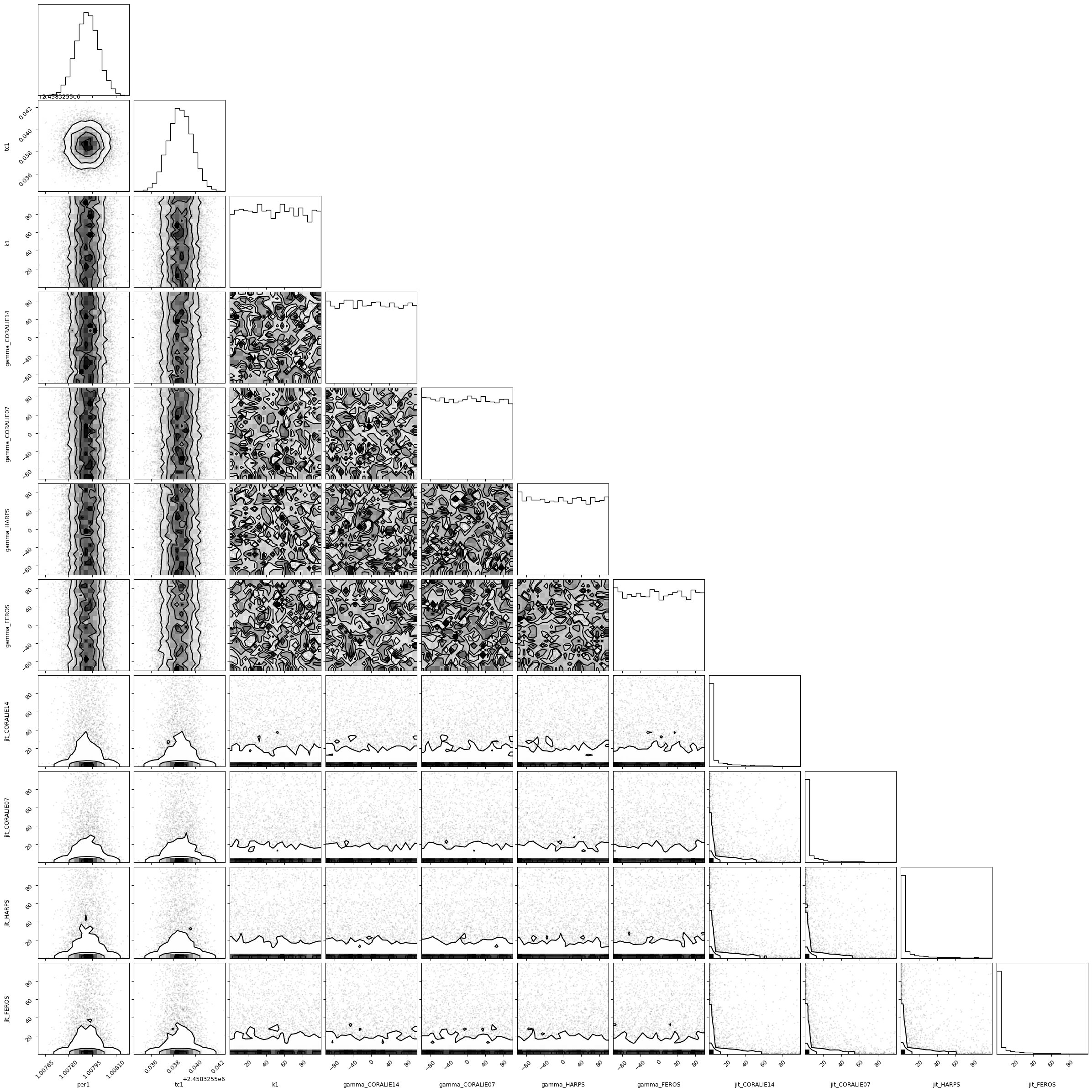
It is always a good idea to draw samples from the posterior to catch errors and see what model predictions are allowed.

prior_samples = model.get_prior_samples(10_000)

import corner
corner.corner(prior_samples)
plt.show()

WARNING:root:Too few points to create valid contours
WARNING:root:Too few points to create valid contours
WARNING:root:Too few points to create valid contours
WARNING:root:Too few points to create valid contours
WARNING:root:Too few points to create valid contours
WARNING:root:Too few points to create valid contours

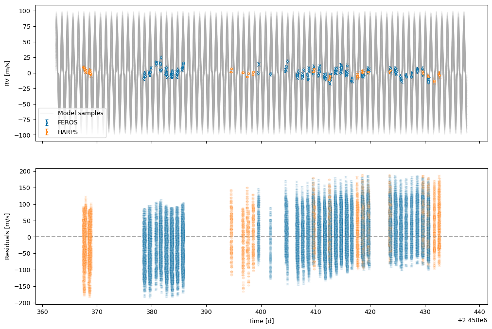
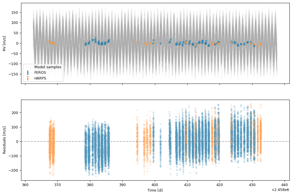
../_images/2216890ca073259681b103369d4dbd4d3d40342d714d8cba908690d3e76b733c.png

sp.plot_rv(model, prior_samples, inst=["FEROS", "HARPS"])
plt.show()

../_images/b365d5520202e5955ac8427a2cf72d629072c0ac3dc958858279b476d2de723d.png

sp.plot_phase(model, prior_samples)
plt.show()

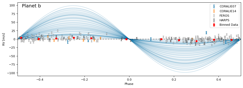
../_images/9d5f5e3b7db7dd6b36eaf70e7f4bb2cc25917553b01c6408c1b99edbe8a187b8.png

As we can see here, the model does not quite capture the variability of the data. However, the period and time are constrained from transits, and there is only so much we can do by varying the semi-amplitude. We will see in the next section how a multi-planet model can improve this, but for now let us sample this single-planet model.

Sampling the Posterior#

from ultranest import ReactiveNestedSampler
from ultranest.stepsampler import SliceSampler, generate_mixture_random_direction

sampler = ReactiveNestedSampler(model.keys(), model.log_likelihood, model.prior_transform)
nsteps = model.ndim * 2
sampler.stepsampler = SliceSampler(
    nsteps=nsteps, generate_direction=generate_mixture_random_direction,
)

DEBUG:ultranest:ReactiveNestedSampler: dims=11+0, resume=False, log_dir=None, backend=hdf5, vectorized=False, nbootstraps=30, ndraw=128..65536

This cell is a tiny hack to silence ultranest output

import logging
# Set root logger
logging.getLogger().setLevel(logging.WARNING)

# Force all existing loggers
for logger_name in logging.root.manager.loggerDict:
    logging.getLogger(logger_name).setLevel(logging.WARNING)

sampler.run(show_status=False);

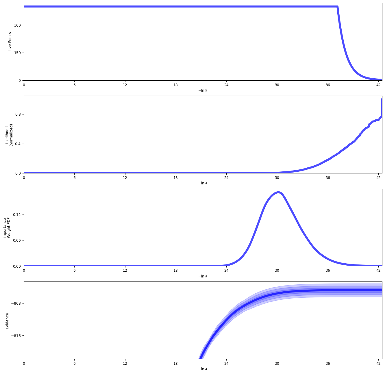
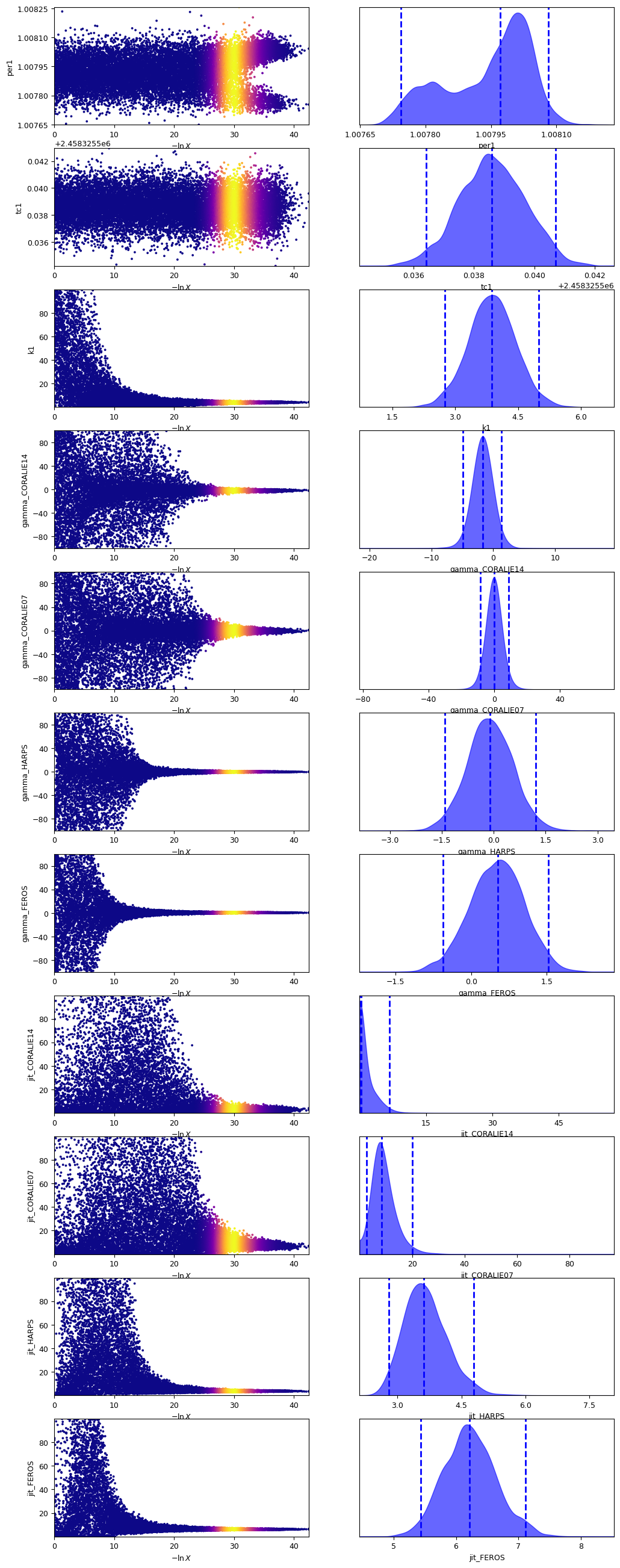
We can first take a look at the nested sampling diagnostic plots.

sampler.plot()
plt.show()

../_images/3b087f49cfbb2a821a5369384839c76901719a894e74b0e352fa60aaa03c0333.png

../_images/314c571f858f675d860dd46e519a831355cd32dd2a92175311aa8cc42883aa5c.png

../_images/749c5c14c09f9fb865d19848c2bd0753e9e7ef645476358d5372007a6321b137.png

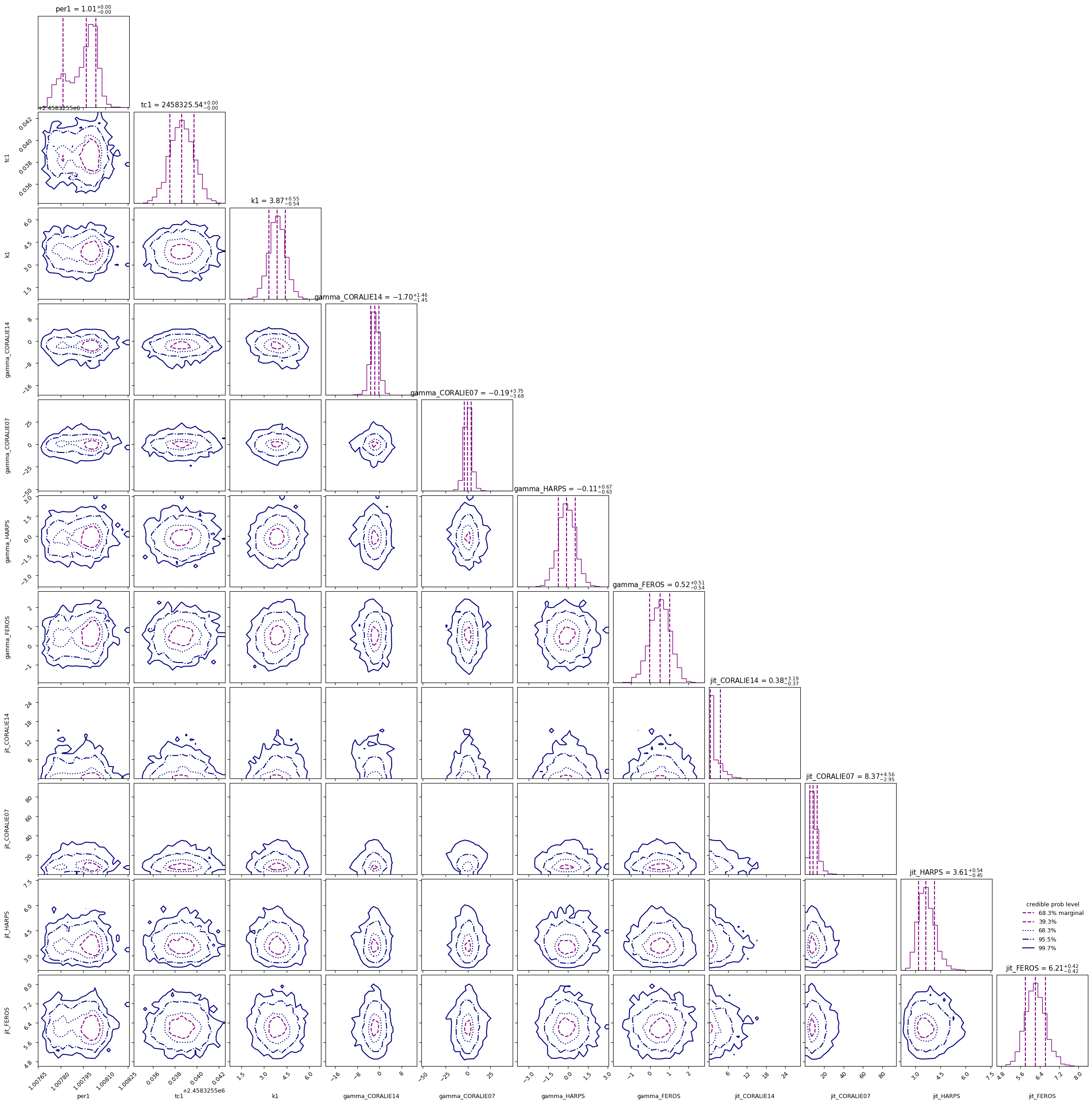
Then we can extract the posterior samples and the evidence.

samples_one = sampler.results["samples"]
lnZ_one = sampler.results["logz"]
lnZerr_one = sampler.results["logzerr"]

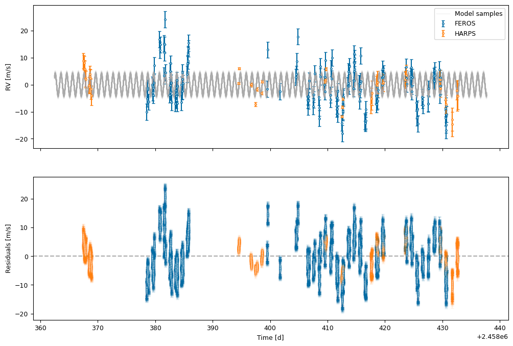
And finally, we can take a look at forward model predictions sampled from the posterior.

sp.plot_rv(model, parameters=samples_one.T, inst=["FEROS", "HARPS"])
plt.show()

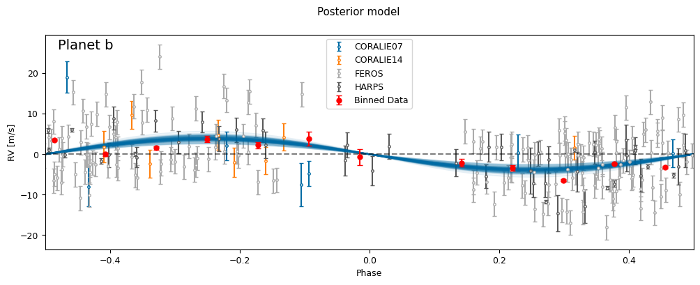
../_images/f5dcafe8bd8351ad3f0d4d7b3ad9f3d17260eefbde082bd0dd2ea2891787a204.png

fig, axs = sp.plot_phase(model, samples_one.T)
fig.suptitle("Posterior model")
plt.show()

../_images/8afad8578917d015e740118ea977d58acfb36f15570359627354c1fb991b18ac.png

Nested Sampling for two Planets#

As we can see above, the single-planet model does not provide a great fit for the data. Let us fit a two-planet model and see how it compares.

Building the Two-Planet Model#

parameters = {
    "per1": sdist.Normal(P, P_err),
    "tc1": sdist.Normal(t0, t0_err),
    "e1": sdist.Fixed(0.0),
    "w1": sdist.Fixed(90.0 * np.pi / 180.0),
    "k1": sdist.Uniform(0.0, 100.0),
    "per2": sdist.Uniform(1.0, 10.0),
    "tc2": sdist.Uniform(2458325.0, 2458330.0),
    "e2": sdist.Fixed(0.0),
    "w2": sdist.Fixed(90.0 * np.pi / 180.0),
    "k2": sdist.Uniform(0.0, 100.0),
    "gamma_CORALIE14": sdist.Uniform(-100.0, 100.0),
    "gamma_CORALIE07": sdist.Uniform(-100.0, 100.0),
    "gamma_HARPS": sdist.Uniform(-100.0, 100.0),
    "gamma_FEROS": sdist.Uniform(-100.0, 100.0),
    "jit_CORALIE14": sdist.LogUniform(1e-3, 100.0),
    "jit_CORALIE07": sdist.LogUniform(1e-3, 100.0),
    "jit_HARPS": sdist.LogUniform(1e-3, 100.0),
    "jit_FEROS": sdist.LogUniform(1e-3, 100.0),
}
model = smod.RVModel(parameters, 2, t, rv, erv, inst=inst, basis="per tc e w k", tmod=tmod)

Prior checks#

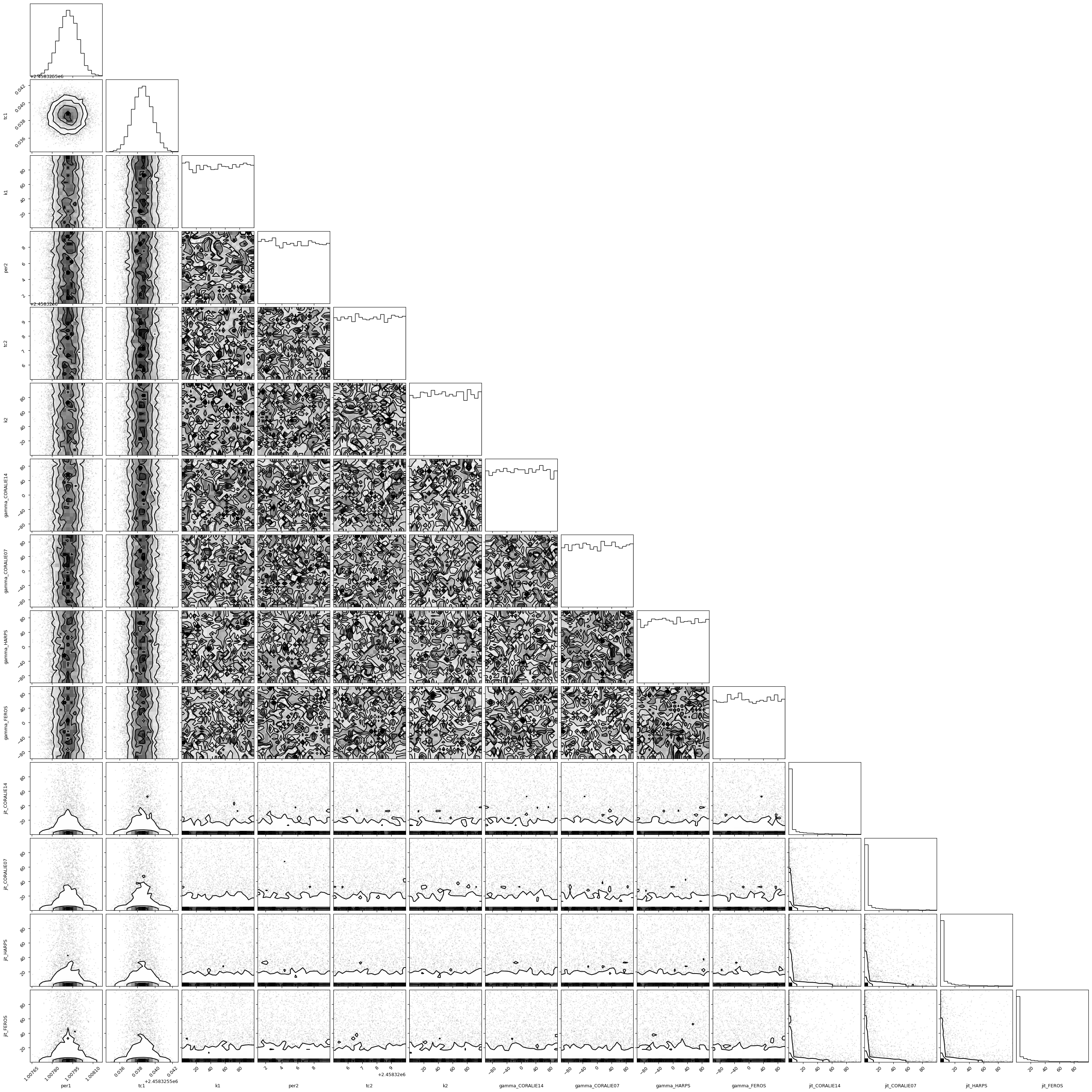
prior_samples = model.get_prior_samples(10_000)

import corner
corner.corner(prior_samples)
plt.show()

WARNING:root:Too few points to create valid contours
WARNING:root:Too few points to create valid contours
WARNING:root:Too few points to create valid contours
WARNING:root:Too few points to create valid contours
WARNING:root:Too few points to create valid contours
WARNING:root:Too few points to create valid contours

../_images/2f2c395639d7ecdaf22967201302b5f533a627a2d1e007e1160de2c004daef55.png

sp.plot_rv(model, prior_samples, inst=["FEROS", "HARPS"])
plt.show()

../_images/fc65443f1dc29a9123db20ea71478361a50bd8c79c1339c6989653fb25d80013.png

MAP Optimization#

test_p = {"per1": P, "tc1": t0, "k1": 10.0}
test_p |= {"per2": 3.0, "tc2": 2458325+2, "k2": 10.0}
for inst_name in model.inst_unique:
    inst_mask = model.inst == inst_name
    test_p[f"gamma_{inst_name}"] = np.mean(model.rv[inst_mask])
    test_p[f"jit_{inst_name}"] = np.mean(model.erv[inst_mask])

from scipy.optimize import minimize
res = minimize(
    lambda p: model.log_prob(p), list(test_p.values()), method='Nelder-Mead',
    options=dict(maxiter=200, maxfev=100000, xatol=1e-8)
)

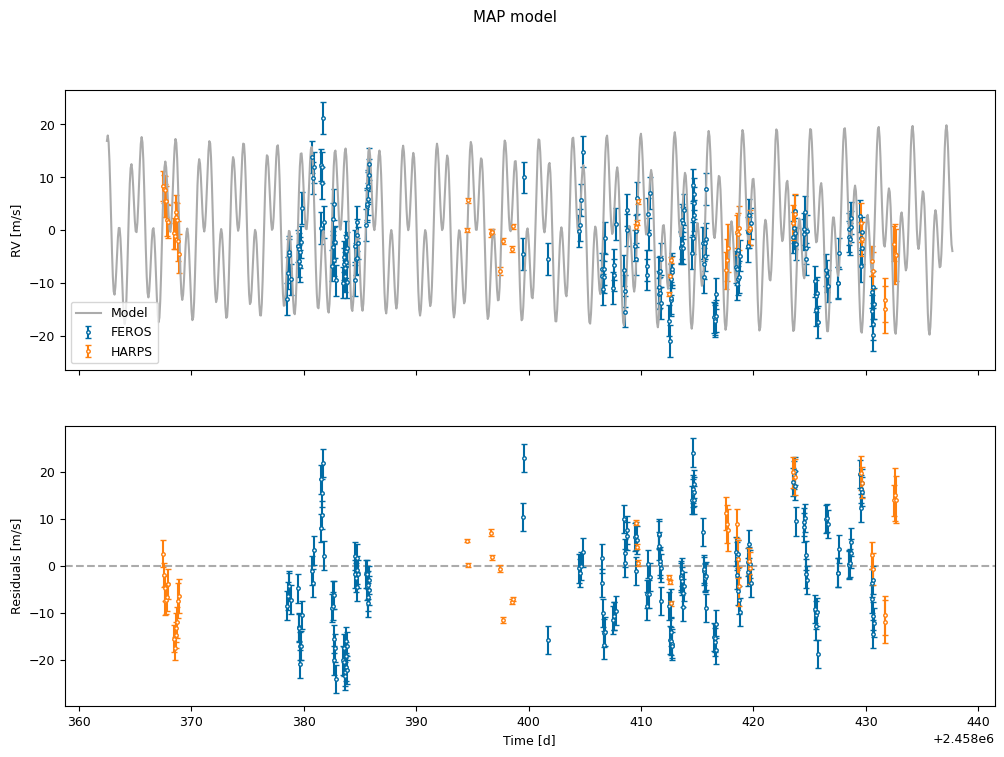
fig, axs = sp.plot_rv(model, parameters=res.x, inst=["FEROS", "HARPS"])
fig.suptitle("MAP model")
plt.show()

../_images/6eb93acb361e8fe4c88739639acf38695eba7955780d91c983cc821947995625.png

fig, axs = sp.plot_phase(model, parameters=res.x)
fig.suptitle("MAP model")
plt.show()

../_images/ffdb5249ea8ddccfda07cc29ba82187622c1a18096bdccf03674e6229f521648.png

Nested Sampling for Two Planets#

sampler = ReactiveNestedSampler(model.keys(), model.log_likelihood, model.prior_transform)
nsteps = model.ndim * 2
sampler.stepsampler = SliceSampler(
    nsteps=nsteps, generate_direction=generate_mixture_random_direction,
)

import logging
# Set root logger
logging.getLogger().setLevel(logging.WARNING)

# Force all existing loggers
for logger_name in logging.root.manager.loggerDict:
    logging.getLogger(logger_name).setLevel(logging.WARNING)

sampler.run(show_status=False);

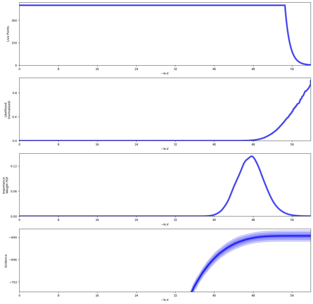
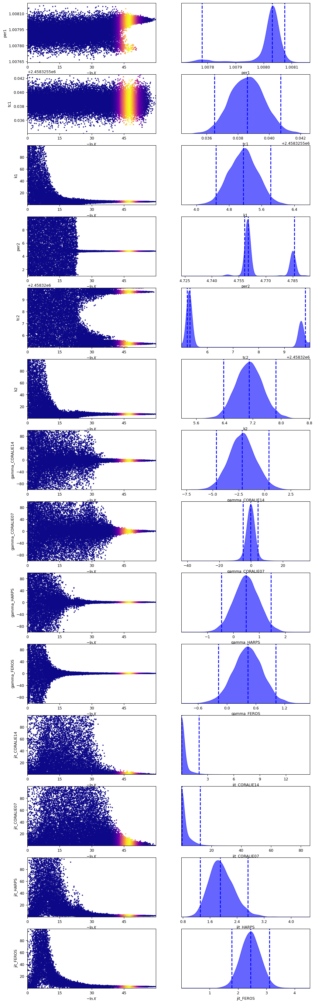
sampler.plot()
plt.show()

../_images/db9b5d33a0128c25f1029b0f6a79b3c6b6cf8a0987addd688e2c3bd77842d101.png

../_images/73ab8d6ad084d407f75fb92589912165514a756db65e214a54ed165ba91d843d.png

../_images/3c201dc35c1812b5c293395bb97e3d25a0ed5bc9b487066084250bf87e27ab40.png

samples_two = sampler.results["samples"]
lnZ_two = sampler.results["logz"]
lnZerr_two = sampler.results["logzerr"]

sp.plot_rv(model, parameters=samples_two.T, inst=["FEROS", "HARPS"])
plt.show()

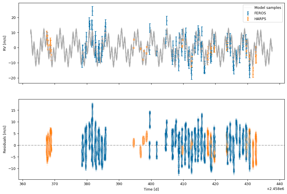
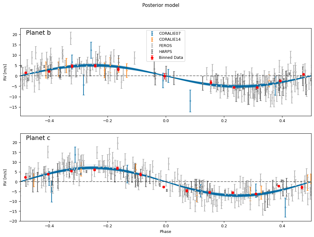
../_images/8cf1ffd3abc0d183eb5b1e192e42753526f8634bd30043f37c75c77d0c2896c7.png

fig, axs = sp.plot_phase(model, samples_two.T)
fig.suptitle("Posterior model")
plt.show()

../_images/02875479c412a90152475a29ae2ee03c8cd293213985b4c34b32789da5e0fdda.png

Model Comparison#

Finally, we can compare the models by calculating the Bayes Factor.

print(f"Log-evidence for one planet: {lnZ_one:.2f} +/- {lnZerr_one:.2f}")
print(f"Log-evidence for two planets: {lnZ_two:.2f} +/- {lnZerr_two:.2f}")
lnK = lnZ_two - lnZ_one
lnKerr = np.sqrt(lnZerr_two**2 + lnZerr_one**2)
print(f"Log-bayes factor for two planets - one planet: {lnK:.2f} +/- {lnKerr:.2f}")

Log-evidence for one planet: -804.80 +/- 0.56
Log-evidence for two planets: -689.62 +/- 0.50
Log-bayes factor for two planets - one planet: 115.18 +/- 0.76

Multi-instrument model with simppler

Contents

Multi-instrument model with `simppler`#

Building the model#

MAP Optimization#

Nested Sampling for a Single Planet#

Prior Samples#

Sampling the Posterior#

Nested Sampling for two Planets#

Building the Two-Planet Model#

Prior checks#

MAP Optimization#

Nested Sampling for Two Planets#

Model Comparison#

Multi-instrument model with simppler

Contents

Multi-instrument model with simppler#

Building the model#

MAP Optimization#

Nested Sampling for a Single Planet#

Prior Samples#

Sampling the Posterior#

Nested Sampling for two Planets#

Building the Two-Planet Model#

Prior checks#

MAP Optimization#

Nested Sampling for Two Planets#

Model Comparison#

Multi-instrument model with `simppler`#